

 * **Undo**: undo the last selection action. The undo step is limited to 10 steps.
* **Reset**: discard all your actions and reset the canvas to its initial state.
### **Mouse Tools**
Four tools from left to right are:


 in front of their feature names. This will allow you to view a summarized expression heatmap for all the selected features. Instead of showing a summarized heatmap, you can explore the co-expression of features by viewing them in different colors (see [Co-expression of Selected Genes](https://stereotoolss-organization.gitbook.io/stereomap-user-manual/bioinformatics-analysis/stereo-seq-t-ff#co-expression-of-selected-genes) for more information).
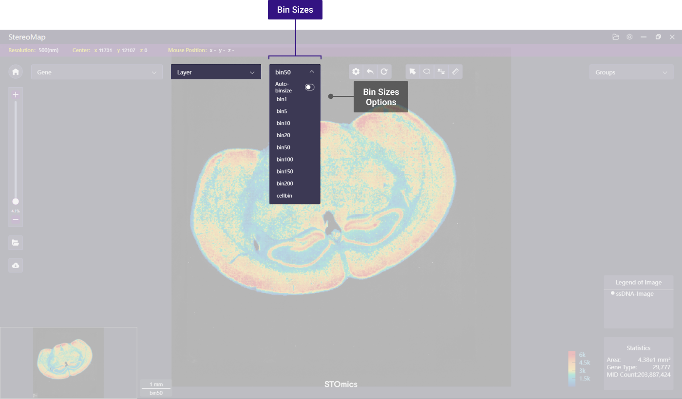
## Layer Menu and Bin Sizes


 in front of the layer name. The windows are linked by the spot coordinates. See [Microorganism and Host Genes](https://stereotoolss-organization.gitbook.io/stereomap-user-manual/bioinformatics-analysis/stereo-seq-n-ffpe#microorganism-and-host-genes) for more information.
* The available bin sizes are 1, 5, 10, 20, 50, 100, 150, 200, and cell bin (only applicable if the dataset contains cell segmentation output). Bin 1 represents one DNB per bin, while Bin 5 represents 5 x 5 DNBs as a binning unit. Cell bin means binning DNBs based on the cell covered regions. There's also an **Auto-binsize** switch that you can toggle. When you turn on the **Auto-binsize** mode, the canvas resolution will automatically adjust based on the zoom-in and zoom-out magnification.
### Main Analysis Layer Display Options
Main analysis layers offer varied display options based on projection type and binning, for easy data exploration.
Options to adjust the display of the heatmap layers:
| Heatmap Options | Explanation | Bin N | Cell Bin |
|---|---|---|---|
| Color | Choose the color scheme of the heatmap for better visualization. |   |   |
| Spot Size | Adjust the spot size. |   | NA |
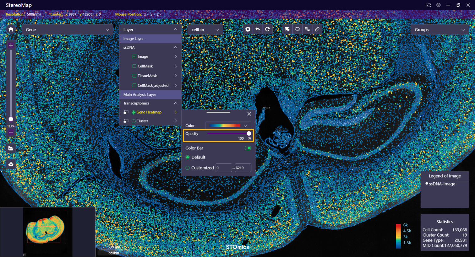
| Opacity | Adjust the heatmap opacity for simultaneously visualize image layers. |   |   |
| MID Filter | Filter spots based on MID count. See MID Filtering for more information.
|   | NA |
| Color Bar | Show or hide the color bar or define the expression range for coloring. By default, the color range goes from 0 to the highest value of any spot in the given bin size. However, you can customize the color range to better visualize bins that fall within a limited feature expression value range. |   |   |
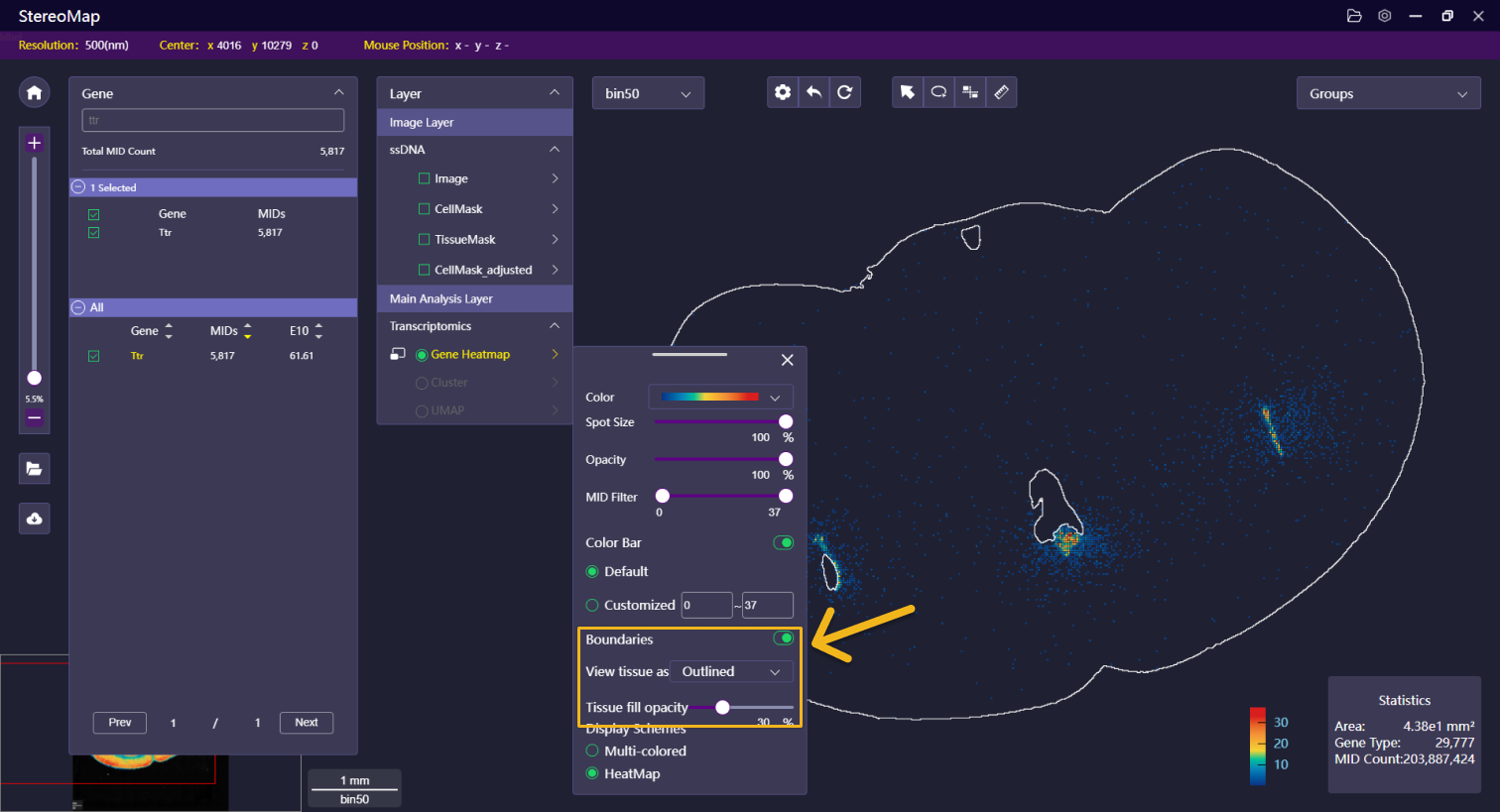
| Boundaries | Show or hide tissue boundary generated from image or expression matrix. The boundary can be displayed as the outline, filled polygon, or both. The opacity of the filled polygon is adjustable. |    | NA |
| Display Schemes | Show expression distribution of features in summarized heatmap or discrete multi-color. See Co-expression of Selected Genes for more information. |   | NA |
| Cluster & UMAP Options | Explanation | Bin N | Cell Bin |
|---|---|---|---|
| Opacity | Adjust the clustering layer opacity for simultaneously visualize image layers. |   |   |
| Form of cells & Outline color | Set cells to appear filled, outlined, or both. The acceptable choices for cell border colors (outlines) include colors assigned by clusters, white, black, and green. | NA |    |


 in front of the cluster name to hide or show the clusters.
* Click the color dot to edit the cluster color.
You can create a new group coupled with the [**Lasso** function](#mouse-tools). Use the lasso to select a region, name the region name, and assign the label to the group. Or you can create new groups by clicking **+ Create a new group** and assign the label to the created new group while saving lasso labels.


 after the group name to edit name or export region coordinates in GeoJSON format. You can also export differential expression analysis required parameters by clicking **GeoJSON for differential expression**. See [Differential Expression Analysis](https://stereotoolss-organization.gitbook.io/stereomap-user-manual/bioinformatics-analysis/stereo-seq-t-ff#differential-expression-analysis) for more information.


